Time Forecasting based on supervised learning
Forecasting model for particle matters (PM2.5)
Background: Existing PM-forecasting systems are highly accurate, but a single run takes a long time and enormous computing resources. This work aimed to cut the computational cost drastically by training a neural network on roughly 100,000 records with minimal resources. It was my undergraduate thesis topic and won the Gold Prize at the KSME Fluid Engineering Division competition (2019).
Data: Hourly data from 2008 to Q3 2018 was collected from Air Korea (air quality) and the Korean open meteorological data portal — 32 variables, 94,225 records, covering air-quality measurements (PM2.5, PM10, NOx, SOx, etc.) and weather variables (temperature, humidity, etc.).
Statistical variable selection & preprocessing: (1) variables with over 50% missing values were dropped to avoid contaminating the later imputation step; (2) AIC (Akaike Information Criterion) with stepwise selection removed variables with low explanatory power for PM2.5 (32 → 21 variables); (3) multicollinearity was removed via VIF — among highly correlated pairs, the physically more fundamental variable was kept based on engineering knowledge (e.g. vapor pressure over relative humidity); (4) the final 13 explanatory variables: PM10, visibility, SO2, CO, NO2, vapor pressure, O3, sea-level pressure, temperature, solar radiation, total cloud, wind direction, wind speed; (5) linear-model imputation produced non-physical values and was rejected — PMM (Predictive Mean Matching) filled the gaps with trends consistent with the measured data.
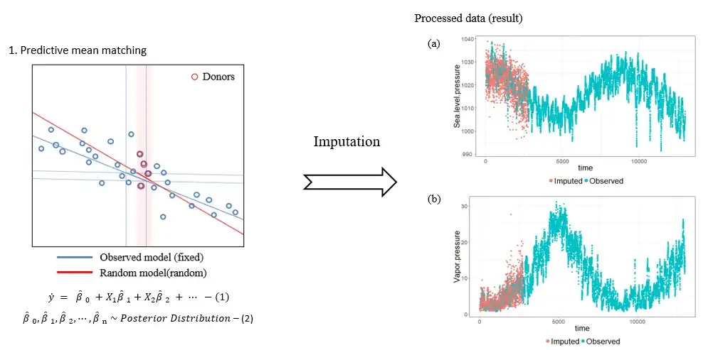
Figure 01. PMM imputation — imputed values (red) follow the trend of observed values (teal)
Model training: A basic ANN with a window-learning scheme — the previous 72 hours of data (selected variables + PM2.5, 14 in total) were reshaped as input (batch size 100) to forecast PM2.5 concentration 6, 12, and 24 hours ahead.
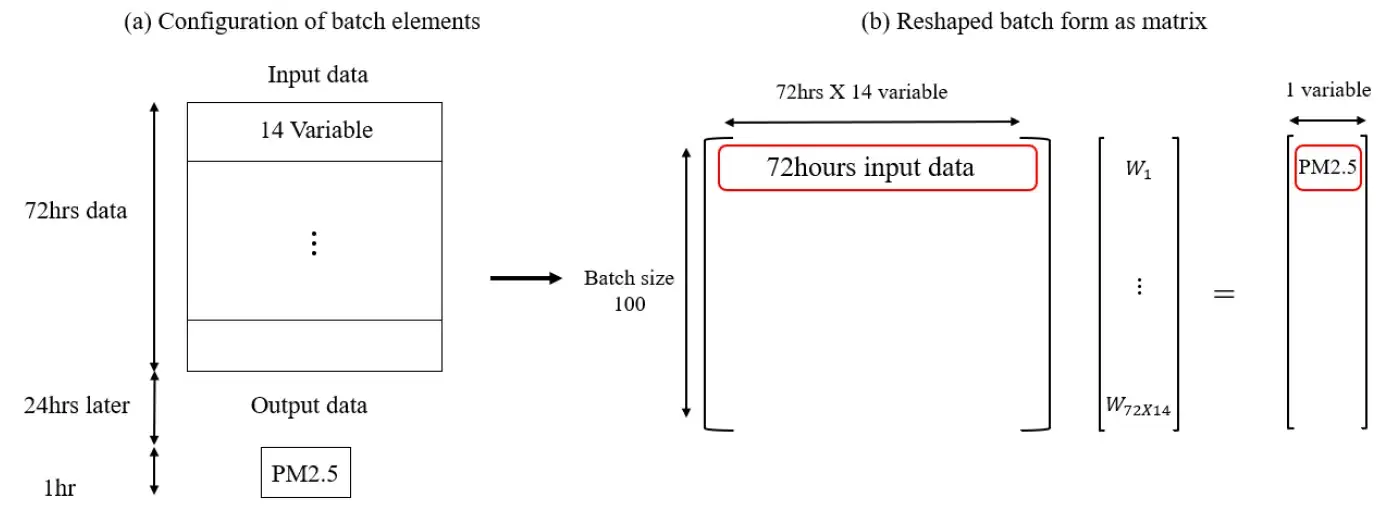
Figure 02. Batch construction — 72 hrs × 14 variables reshaped as a matrix input (batch size 100)
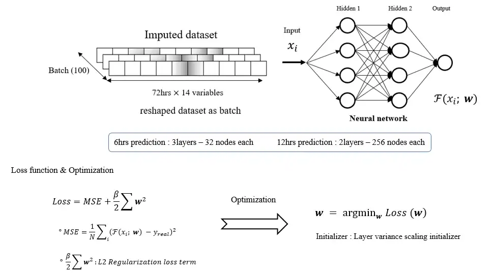
Figure 03. Network structure & loss — 6-hr model: 3 layers × 32 nodes, 12-hr model: 2 layers × 256 nodes, Loss = MSE + L2 regularization
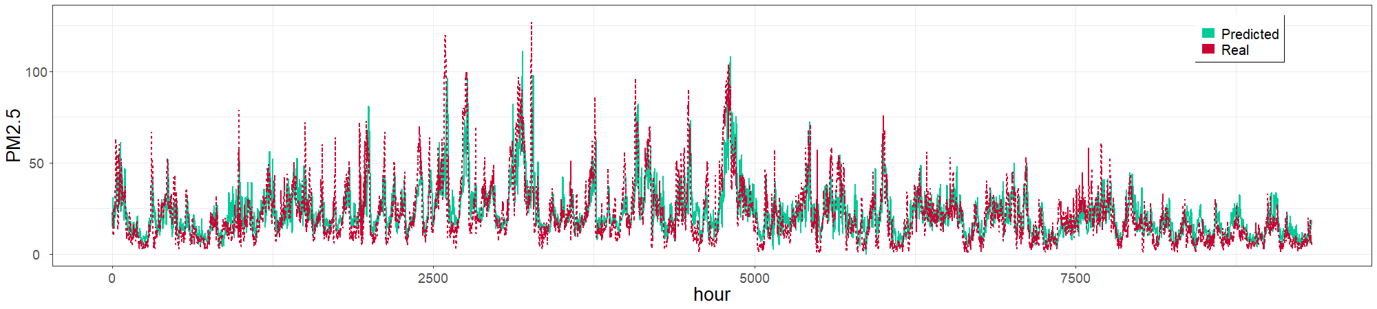
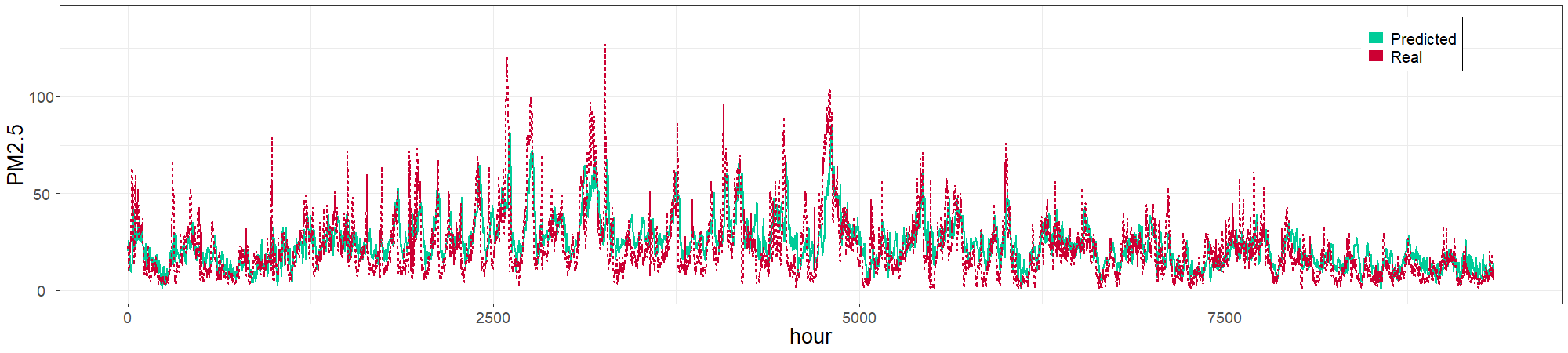
Figure 04. 6hrs (top) and 12hrs (bottom) forecasts
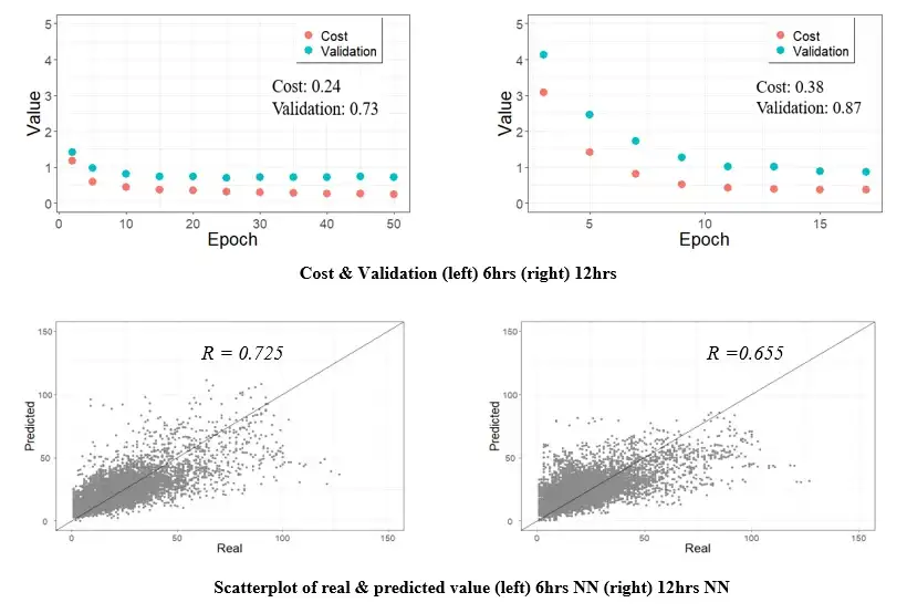
Figure 05. Training curves and real-vs-predicted scatter — R=0.725 (6 hrs), R=0.655 (12 hrs)
Results, limitations & follow-up: The time-series plots above show the 6-hour and 12-hour forecasts, with real-vs-predicted correlation of R=0.725 (6 hrs) and R=0.655 (12 hrs); at the time, the 6-hour model appeared to perform best. Later analysis, however, revealed a time-lag phenomenon — the prediction curve trails the measured values — a structural limitation of training on simple Euclidean (error-distance) loss. Performance also degraded toward high-concentration regimes. To compensate, a follow-up experiment in graduate school (2021) applied reinforcement learning that reflects the slope (angle) of the error in addition to its magnitude, confirming partial improvement.
Presented at the KSME 2019 Autumn Annual Conference.
Gold Prize, KSME Fluid Engineering Division Competition (2019).